

Vision Models (Notebook)#
CNN Flower Classification#
Author: Valentina Staneva

This notebook demonstrates training a CNN model to classify flower images.
This notebook is built on the Tensorflow Image Classification tutorial.

Outline#
The notebook goes through the following workflow:
Read a dataset of flower images and prepare for training, validation, and testing
Train a basic dense model
Train a CNN model
Incorporate a data augmentation strategy
Test model performance on the held out dataset
Setup#
⚠️ Warning: This notebook runs significanlty faster on GPU. You can select a GPU in Colab by navigating to Runtime -> Change Runtime Type -> T4. A100 is way faster but it may eat up your free tier quickly. Note, when you change your runtime your notebook need to be restarted, so do it before you execute any cells.
import os
os.environ["KERAS_BACKEND"] = "torch"
import matplotlib.pyplot as plt
import numpy as np
import PIL

import keras
from keras import layers
from keras.models import Sequential
# set random seed for result reproducibility
keras.utils.set_random_seed(123)
Flowers Dataset#
This tutorial uses a dataset of about 3,700 photos of flowers. The dataset contains five types of flowers:
  daisy
  dandelion
  roses
  sunflowers
  tulips
The goal is to build a classifier which predicts the type of flowers in new images.
The dataset is part of a collection of datasets in the tensorflow library which can be directly loaded.
# downloading images

import pathlib
dataset_url = "https://storage.googleapis.com/download.tensorflow.org/example_images/flower_photos.tgz"
data_dir = keras.utils.get_file('flower_photos.tar', origin=dataset_url, extract=True)
data_dir = pathlib.Path(data_dir).with_suffix('')
print(data_dir)

image_count = len(list(data_dir.glob('*/*.jpg')))
print(image_count)
/root/.keras/datasets/flower_photos_extracted
0
ls /root/.keras/datasets/flower_photos_extracted/flower_photos
daisy/ dandelion/ LICENSE.txt roses/ sunflowers/ tulips/
We note that the images are arranged in folders with their names.
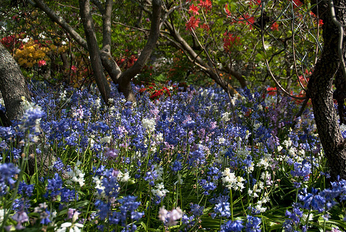
# looking at a few tulips
tulips = list(sorted(data_dir.glob('flower_photos/tulips/*')))
PIL.Image.open(str(tulips[1]))
Images are not the same size!
The images in the dataset are not the same size so we will resize them so that it is easier to put them in an array and process them efficiently. We fix the weight and height to be 150 (this will distort the images a bit but we want to see if the algorithm can be robust to some stretching). Resizing can be achieved automatically while reading the data with the keras.utils.image_dataset_from_directory function and setting the image size. This function can do a few extra steps for us:
split the data into two subsets: training and testing
infer the labels come from the name of the folders and put them in categorical format
HEIGHT = 150
WIDTH = 150
train_ds, test_ds = keras.utils.image_dataset_from_directory(
  data_dir / "flower_photos",
  validation_split=0.2,
  subset="both",
  labels="inferred",
  label_mode="categorical",
  seed=123,
  image_size=(HEIGHT, WIDTH),
)
Found 3670 files belonging to 5 classes.
Using 2936 files for training.
Using 734 files for validation.
📝 Note: If resizing images in your dataset, you need to select an approach which does not distort substantially your data. The keras.utils.image_dataset_from_directory function has some other options such as cropping or padding to aspect ratio. In your research, you may need write your own functions which are appropriate for your data.
# help(keras.utils.image_dataset_from_directory)
Held-out test set#
Note we set aside 20% for a test set which we will NOT use in model training and selection. It is easy to overfit the model performance to the specific test we have selected and because we have no more “unseen” data to test on, our measures of performance may be skewed. We will only use the test set in the end to evaluate the performance on “unseen” data.
📝 Note: While the loading function called the split “validation”, the way we are treating it determines its name: if we are only using it in the end, and we do not have any other flower data to test on, then it is a “test” set, while if we are using it for experimentation, then it is a “validations” set. Occasionally, you will find this terminology reversed, but we will stick to these definitions here.
⚠️ Warning: When splitting a dataset, we should also be careful how our data are ordered. By default, this function is shuffling the data before splitting, so we will not get only one type of flowers in the test set. In practice, you may want to design your own validation strategy, and you may need to define your own splitting functions, but this will give you full control over your experiments.
The output data format is organized in batches which is good for efficiency, but since this dataset is not big and we want to simplify the structure we will convert it to numpy arrays.
list(train_ds.unbatch())[1][1]
<tf.Tensor: shape=(5,), dtype=float32, numpy=array([0., 0., 0., 1., 0.], dtype=float32)>
# convert to numpy arrays
train_images, train_labels = zip(*list(train_ds.unbatch()))
train_images = np.array(train_images)
train_labels = np.array(train_labels)
print(train_images.shape)
print(train_labels.shape)
(2936, 150, 150, 3)
(2936, 5)
We loaded the labels in a categorical format, but we also need the class names. These correspond to the directory names in alphabetical order.
class_names = ["daisy", "dandelion", "roses", "sunflowers","tulips"]
num_classes = len(class_names)
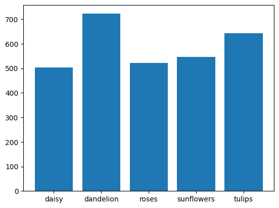
Let’s see the distribution of the classes:
plt.bar(class_names, train_labels.sum(axis=0))
<BarContainer object of 5 artists>
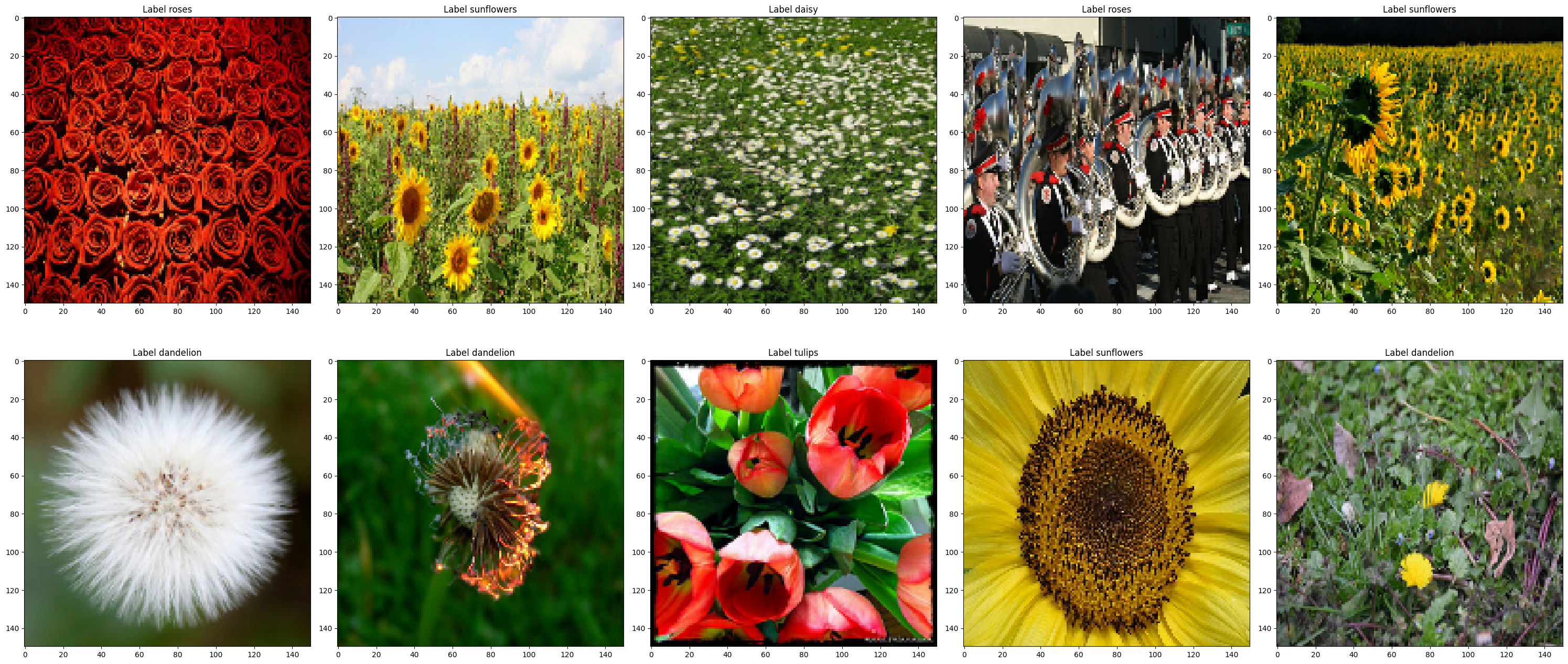
Visualize the data#
plt.rcParams["figure.figsize"] = [30, 15]
plt.rcParams["figure.autolayout"] = True

counter = 0
for image, label in zip(train_images, train_labels):
  plt.subplot(2, 5, counter+1)
  plt.imshow(image.astype("uint8"))
  label_name = class_names[np.where(label==1)[0][0]]
  plt.title('Label {}'.format(label_name))
  counter += 1
  if counter == 10:
    break
Rescale the data#
The RGB channel values are in the [0, 255] range. This is not ideal for a neural network; in general you should seek to make your input values small.
We can rescale values to be in the [0, 1] range by using tf.keras.layers.Rescaling in the model definition itself.
layers.Rescaling(1./255)
<Rescaling name=rescaling, built=False>
Dense Model#
from keras.layers import Input, Dense, Flatten, Rescaling, Conv2D, MaxPooling2D
# Define a dense neural network with one hidden layer
output_dim = train_labels.shape[1]
hidden_dim = 50

dense_model = keras.Sequential()
dense_model.add(Input(shape = (HEIGHT, WIDTH, 3)))
dense_model.add(Flatten())
dense_model.add(Rescaling(1./255))
dense_model.add(Dense(hidden_dim, activation="relu"))
dense_model.add(Dense(output_dim, activation="softmax"))
dense_model.summary()
Model: "sequential"
┏━━━━━━━━━━━━━━━━━━━━━━━━━━━━━━━━━┳━━━━━━━━━━━━━━━━━━━━━━━━┳━━━━━━━━━━━━━━━┓
┃ Layer (type)                    ┃ Output Shape           ┃       Param # ┃
┡━━━━━━━━━━━━━━━━━━━━━━━━━━━━━━━━━╇━━━━━━━━━━━━━━━━━━━━━━━━╇━━━━━━━━━━━━━━━┩
│ flatten (Flatten)               │ (None, 67500)          │             0 │
├─────────────────────────────────┼────────────────────────┼───────────────┤
│ rescaling_1 (Rescaling)         │ (None, 67500)          │             0 │
├─────────────────────────────────┼────────────────────────┼───────────────┤
│ dense (Dense)                   │ (None, 50)             │     3,375,050 │
├─────────────────────────────────┼────────────────────────┼───────────────┤
│ dense_1 (Dense)                 │ (None, 5)              │           255 │
└─────────────────────────────────┴────────────────────────┴───────────────┘
Total params: 3,375,305 (12.88 MB)
Trainable params: 3,375,305 (12.88 MB)
Non-trainable params: 0 (0.00 B)
# Define the loss and the evaluation metrics
dense_model.compile(optimizer=keras.optimizers.Adam(learning_rate=0.0001),
              loss='categorical_crossentropy',
              metrics=['accuracy'])
Early Stopping: We set the max number of epochs to 50 in the Model.fit method, but we will also set an early stopping criterion which will monitor how the algorithm performs on the validation set, and if there is no significant improvement, the algorithm will stop.
from keras.callbacks import EarlyStopping
es = EarlyStopping(monitor='val_loss', mode='min', patience=5,  restore_best_weights=True)
📝 Note: Here we select to monitor the validation loss. Our actual goal is to have high validation accuracy, but the accuracy metric can be very noisy for a small validation set, so in practice it can be more stable to monitor the validation loss.
%%time
# Fit the model
history = dense_model.fit(train_images,
                          train_labels,
                          validation_split=0.2,
                          epochs=50,
                          batch_size=32,
                          callbacks=[es]
                          )
Epoch 1/50
74/74 ━━━━━━━━━━━━━━━━━━━━ 1s 16ms/step - accuracy: 0.3228 - loss: 1.5930 - val_accuracy: 0.3912 - val_loss: 1.4189
Epoch 2/50
74/74 ━━━━━━━━━━━━━━━━━━━━ 1s 16ms/step - accuracy: 0.4434 - loss: 1.3427 - val_accuracy: 0.4031 - val_loss: 1.4268
Epoch 3/50
74/74 ━━━━━━━━━━━━━━━━━━━━ 1s 19ms/step - accuracy: 0.5072 - loss: 1.2198 - val_accuracy: 0.4099 - val_loss: 1.4025
Epoch 4/50
74/74 ━━━━━━━━━━━━━━━━━━━━ 1s 20ms/step - accuracy: 0.5311 - loss: 1.1551 - val_accuracy: 0.4218 - val_loss: 1.3369
Epoch 5/50
74/74 ━━━━━━━━━━━━━━━━━━━━ 1s 17ms/step - accuracy: 0.5686 - loss: 1.1018 - val_accuracy: 0.4456 - val_loss: 1.3222
Epoch 6/50
74/74 ━━━━━━━━━━━━━━━━━━━━ 1s 16ms/step - accuracy: 0.5745 - loss: 1.0944 - val_accuracy: 0.4082 - val_loss: 1.4156
Epoch 7/50
74/74 ━━━━━━━━━━━━━━━━━━━━ 1s 16ms/step - accuracy: 0.5703 - loss: 1.0644 - val_accuracy: 0.4371 - val_loss: 1.3762
Epoch 8/50
74/74 ━━━━━━━━━━━━━━━━━━━━ 1s 16ms/step - accuracy: 0.5975 - loss: 1.0205 - val_accuracy: 0.4354 - val_loss: 1.3882
Epoch 9/50
74/74 ━━━━━━━━━━━━━━━━━━━━ 1s 17ms/step - accuracy: 0.6193 - loss: 0.9891 - val_accuracy: 0.4252 - val_loss: 1.4200
Epoch 10/50
74/74 ━━━━━━━━━━━━━━━━━━━━ 1s 16ms/step - accuracy: 0.6231 - loss: 0.9848 - val_accuracy: 0.4388 - val_loss: 1.3739
CPU times: user 12.5 s, sys: 337 ms, total: 12.9 s
Wall time: 12.8 s
plt.rcParams["figure.figsize"] = [10, 5]
plt.rcParams["figure.autolayout"] = True
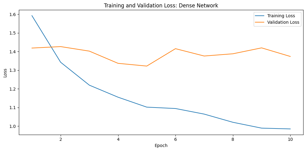
# accuracy metrics at each iteration are stored in the history variable
acc = history.history['accuracy']
val_acc = history.history['val_accuracy']

loss = history.history['loss']
val_loss = history.history['val_loss']

epochs_range = range(1, len(history.history['loss'])+1)

# Loss
plt.plot(epochs_range, loss, label='Training Loss')
plt.plot(epochs_range, val_loss, label='Validation Loss')
plt.legend(loc='upper right')
plt.title('Training and Validation Loss: Dense Network')
plt.xlabel('Epoch')
plt.ylabel('Loss')
plt.show()

# Accuracy
plt.plot(epochs_range, acc, label='Training Accuracy')
plt.plot(epochs_range, val_acc, label='Validation Accuracy')
plt.legend(loc='lower right')
plt.title('Training and Validation Accuracy: Dense Network')
plt.xlabel('Epoch')
plt.ylabel('Accuracy')
Text(0, 0.5, 'Accuracy')
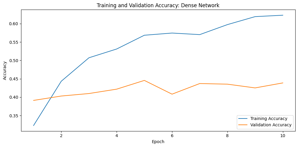
Performance is not very good! Since flowers in the images are not centered, it is hard for a dense linear network to learn how to match the color in one image to the corresponding color in another image. Since there are way more parameters that observation the network can overfit on the training data but cannot predict on the validation data.
CNN Model#
Create the model#
The Keras Sequential model consists of three convolution blocks (keras.layers.Conv2D) with a max pooling layer (keras.layers.MaxPooling2D) in each of them. There’s a fully-connected layer (keras.layers.Dense) with 128 units on top of it that is activated by a ReLU activation function ('relu'). This model has not been tuned for high accuracy; the goal of this tutorial is to show a standard approach.
cnn_model = Sequential([
  layers.Input(shape = (HEIGHT, WIDTH, 3)),
  layers.Rescaling(1./255),

  layers.Conv2D(filters=16, kernel_size=3, padding='same', activation='relu'),
  layers.MaxPooling2D(),

  layers.Conv2D(filters=32, kernel_size=3, padding='same', activation='relu'),
  layers.MaxPooling2D(),

  layers.Conv2D(filters=64, kernel_size=3, padding='same', activation='relu'),
  layers.MaxPooling2D(),

  layers.Conv2D(filters=128, kernel_size=3, padding='same', activation='relu'),
  layers.MaxPooling2D(),

  layers.Flatten(),
  layers.Dense(128, activation='relu'),

  layers.Dense(num_classes, name="outputs", activation='softmax')
])
View all the layers of the network using the Keras Model.summary method:
cnn_model.summary()
Model: "sequential_1"
┏━━━━━━━━━━━━━━━━━━━━━━━━━━━━━━━━━┳━━━━━━━━━━━━━━━━━━━━━━━━┳━━━━━━━━━━━━━━━┓
┃ Layer (type)                    ┃ Output Shape           ┃       Param # ┃
┡━━━━━━━━━━━━━━━━━━━━━━━━━━━━━━━━━╇━━━━━━━━━━━━━━━━━━━━━━━━╇━━━━━━━━━━━━━━━┩
│ rescaling_2 (Rescaling)         │ (None, 150, 150, 3)    │             0 │
├─────────────────────────────────┼────────────────────────┼───────────────┤
│ conv2d (Conv2D)                 │ (None, 150, 150, 16)   │           448 │
├─────────────────────────────────┼────────────────────────┼───────────────┤
│ max_pooling2d (MaxPooling2D)    │ (None, 75, 75, 16)     │             0 │
├─────────────────────────────────┼────────────────────────┼───────────────┤
│ conv2d_1 (Conv2D)               │ (None, 75, 75, 32)     │         4,640 │
├─────────────────────────────────┼────────────────────────┼───────────────┤
│ max_pooling2d_1 (MaxPooling2D)  │ (None, 37, 37, 32)     │             0 │
├─────────────────────────────────┼────────────────────────┼───────────────┤
│ conv2d_2 (Conv2D)               │ (None, 37, 37, 64)     │        18,496 │
├─────────────────────────────────┼────────────────────────┼───────────────┤
│ max_pooling2d_2 (MaxPooling2D)  │ (None, 18, 18, 64)     │             0 │
├─────────────────────────────────┼────────────────────────┼───────────────┤
│ conv2d_3 (Conv2D)               │ (None, 18, 18, 128)    │        73,856 │
├─────────────────────────────────┼────────────────────────┼───────────────┤
│ max_pooling2d_3 (MaxPooling2D)  │ (None, 9, 9, 128)      │             0 │
├─────────────────────────────────┼────────────────────────┼───────────────┤
│ flatten_1 (Flatten)             │ (None, 10368)          │             0 │
├─────────────────────────────────┼────────────────────────┼───────────────┤
│ dense_2 (Dense)                 │ (None, 128)            │     1,327,232 │
├─────────────────────────────────┼────────────────────────┼───────────────┤
│ outputs (Dense)                 │ (None, 5)              │           645 │
└─────────────────────────────────┴────────────────────────┴───────────────┘
Total params: 1,425,317 (5.44 MB)
Trainable params: 1,425,317 (5.44 MB)
Non-trainable params: 0 (0.00 B)
For this tutorial, choose the keras.optimizers.Adam optimizer and categorical_crossentropy loss function. To view training and validation accuracy for each training epoch, pass the metrics argument to Model.compile.
cnn_model.compile(optimizer='adam',
              loss='categorical_crossentropy',
              metrics=['accuracy'])
📝 Note: One can pass other built-in metrics or pass their own metric function.
Train the model#
from keras.callbacks import EarlyStopping
es = EarlyStopping(monitor='val_loss', mode='min', patience=10,  restore_best_weights=True)
# caluclate how many iterations are there in one epoch
print(train_labels.shape)
2936*0.8/64
(2936, 5)
36.7
%%time
# thise step takes <1 min.
epochs=50
history = cnn_model.fit(
  train_images,
  train_labels,
  validation_split=0.2,
  epochs=epochs,
  batch_size=64,
  callbacks=[es]
)
Epoch 1/50
37/37 ━━━━━━━━━━━━━━━━━━━━ 2s 50ms/step - accuracy: 0.3169 - loss: 1.4927 - val_accuracy: 0.4422 - val_loss: 1.3689
Epoch 2/50
37/37 ━━━━━━━━━━━━━━━━━━━━ 2s 51ms/step - accuracy: 0.5302 - loss: 1.1692 - val_accuracy: 0.5102 - val_loss: 1.2243
Epoch 3/50
37/37 ━━━━━━━━━━━━━━━━━━━━ 2s 51ms/step - accuracy: 0.5826 - loss: 1.0361 - val_accuracy: 0.5833 - val_loss: 1.0907
Epoch 4/50
37/37 ━━━━━━━━━━━━━━━━━━━━ 2s 47ms/step - accuracy: 0.6350 - loss: 0.9335 - val_accuracy: 0.6003 - val_loss: 1.0492
Epoch 5/50
37/37 ━━━━━━━━━━━━━━━━━━━━ 2s 48ms/step - accuracy: 0.6691 - loss: 0.8483 - val_accuracy: 0.6105 - val_loss: 1.0004
Epoch 6/50
37/37 ━━━━━━━━━━━━━━━━━━━━ 2s 48ms/step - accuracy: 0.7134 - loss: 0.7491 - val_accuracy: 0.6310 - val_loss: 0.9745
Epoch 7/50
37/37 ━━━━━━━━━━━━━━━━━━━━ 2s 47ms/step - accuracy: 0.7394 - loss: 0.7154 - val_accuracy: 0.6173 - val_loss: 1.0462
Epoch 8/50
37/37 ━━━━━━━━━━━━━━━━━━━━ 2s 47ms/step - accuracy: 0.7734 - loss: 0.6024 - val_accuracy: 0.6463 - val_loss: 1.0132
Epoch 9/50
37/37 ━━━━━━━━━━━━━━━━━━━━ 2s 51ms/step - accuracy: 0.8207 - loss: 0.4929 - val_accuracy: 0.6310 - val_loss: 1.1057
Epoch 10/50
37/37 ━━━━━━━━━━━━━━━━━━━━ 2s 50ms/step - accuracy: 0.8526 - loss: 0.4112 - val_accuracy: 0.6429 - val_loss: 1.1077
Epoch 11/50
37/37 ━━━━━━━━━━━━━━━━━━━━ 2s 47ms/step - accuracy: 0.8854 - loss: 0.3380 - val_accuracy: 0.6531 - val_loss: 1.2112
Epoch 12/50
37/37 ━━━━━━━━━━━━━━━━━━━━ 2s 48ms/step - accuracy: 0.9195 - loss: 0.2411 - val_accuracy: 0.6548 - val_loss: 1.3456
Epoch 13/50
37/37 ━━━━━━━━━━━━━━━━━━━━ 2s 47ms/step - accuracy: 0.9463 - loss: 0.1717 - val_accuracy: 0.6548 - val_loss: 1.5005
Epoch 14/50
37/37 ━━━━━━━━━━━━━━━━━━━━ 2s 47ms/step - accuracy: 0.9651 - loss: 0.1191 - val_accuracy: 0.6480 - val_loss: 1.5866
Epoch 15/50
37/37 ━━━━━━━━━━━━━━━━━━━━ 2s 47ms/step - accuracy: 0.9685 - loss: 0.1048 - val_accuracy: 0.6429 - val_loss: 1.7212
Epoch 16/50
37/37 ━━━━━━━━━━━━━━━━━━━━ 2s 52ms/step - accuracy: 0.9698 - loss: 0.1066 - val_accuracy: 0.6327 - val_loss: 1.8781
CPU times: user 29 s, sys: 291 ms, total: 29.3 s
Wall time: 29.2 s
⚠️ Warning: If you run the fit command twice the model will continue to update the existing model, unless you rerun the model definition command.
We observe that
the training set accuracy is almost 1
the validation set accuracy is around ~0.63.
Visualize training results#
Create plots of the loss and accuracy on the training and validation sets:
plt.rcParams["figure.figsize"] = [10, 5]
plt.rcParams["figure.autolayout"] = True
# accuracy metrics at each iteration are stored in the history variable
acc = history.history['accuracy']
val_acc = history.history['val_accuracy']

loss = history.history['loss']
val_loss = history.history['val_loss']

epochs_range = range(1, len(history.history['loss'])+1)

# Loss
plt.plot(epochs_range, loss, label='Training Loss')
plt.plot(epochs_range, val_loss, label='Validation Loss')
plt.legend(loc='upper right')
plt.title('Training and Validation Loss: Base')
plt.xlabel('Epoch')
plt.ylabel('Loss')
plt.show()

# Accuracy
plt.plot(epochs_range, acc, label='Training Accuracy')
plt.plot(epochs_range, val_acc, label='Validation Accuracy')
plt.legend(loc='lower right')
plt.title('Training and Validation Accuracy: Base')
plt.xlabel('Epoch')
plt.ylabel('Accuracy')
Text(0, 0.5, 'Accuracy')
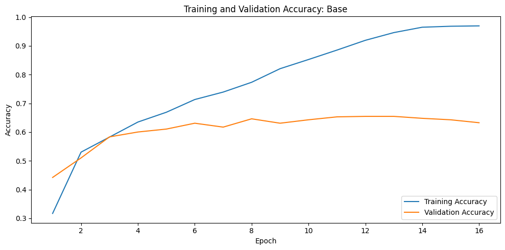
The plots show that training accuracy and validation accuracy are off by large margins, and the model has achieved around 60% accuracy on the validation set. Better than before, but still space for improvement.
The next two sections of the tutorial show some strategies how to avoid some of the overfitting challenges.
🧑💻 Exercise: Add one more 2D convolutional layer to the existing model. Retrain the model and visualize the performance. What do you observe? Name your model deeper_cnn_model so that you save it as a separate variable.
# define a model as above with one extra convolutional layer with 256 filters
# deeper_cnn_model = ...
# set the loss and the optimizer
# ...
# train the model
# ...
# plot the loss and the accuracy
# ...
Model Improvements#
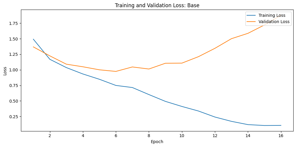
In the plots above, the training accuracy is increasing linearly over time, whereas validation accuracy stalls around 60% in the training process. Also, the difference in accuracy between training and validation accuracy is noticeable—a sign of overfitting.
When there are a small number of training examples, the model sometimes learns from noises or unwanted details from training examples—to an extent that it negatively impacts the performance of the model on new examples. It means that the model will have a difficult time generalizing on a new dataset.
There are multiple ways to fight overfitting in the training process and we will discuss those below.
Data Augmentation#
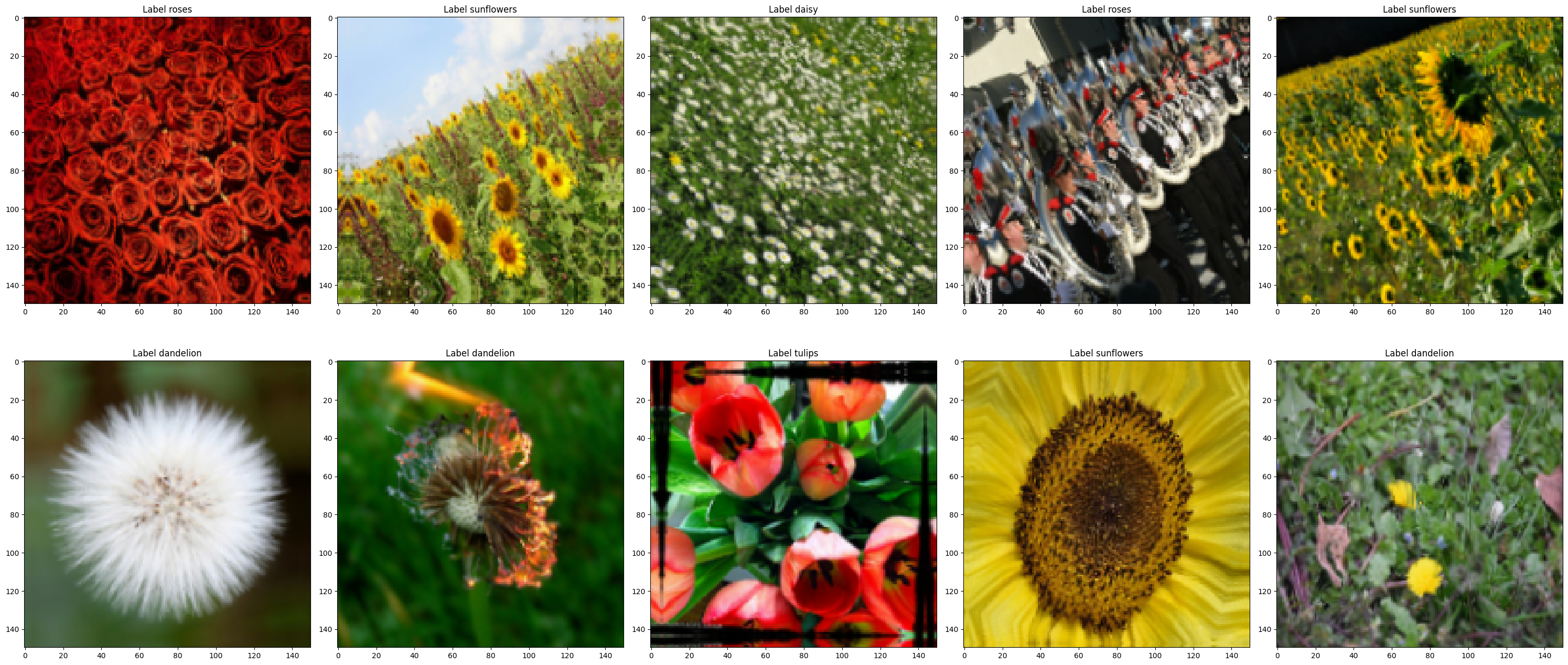
Data augmentation takes the approach of generating additional training data from your existing examples by augmenting them using random transformations that yield believable-looking images. This helps expose the model to more aspects of the data and generalize better.
We will implement data augmentation using the following Keras preprocessing layers: keras.layers.RandomFlip, keras.layers.RandomRotation, and keras.layers.RandomZoom. These can be included inside your model like other layers, and run on the GPU.
Visualize a few augmented examples by applying data augmentation to the same image several times:
data_augmentation = keras.Sequential(
  [
    layers.RandomFlip("horizontal"),
    layers.RandomRotation(0.1),
    layers.RandomZoom(0.1),
  ]
)
plt.rcParams["figure.figsize"] = [30, 15]
plt.rcParams["figure.autolayout"] = True

counter = 0
for image, label in zip(train_images, train_labels):
  plt.subplot(2, 5, counter+1)
  data_augmentation(np.reshape(image, (1, HEIGHT, WIDTH, 3)))
  plt.imshow(data_augmentation(np.reshape(image, (1, HEIGHT, WIDTH, 3))).cpu().numpy().astype('uint8').squeeze())
  label_name = class_names[np.where(label==1)[0][0]]
  plt.title('Label {}'.format(label_name))
  counter += 1
  if counter == 10:
    break
# help(layers.RandomRotation)
We will add data augmentation to your model before training in the next step.
cnn_model_aug = Sequential([
  data_augmentation,
  layers.Rescaling(1./255),

  layers.Conv2D(16, 3, padding='same', activation='relu'),
  layers.MaxPooling2D(),

  layers.Conv2D(32, 3, padding='same', activation='relu'),
  layers.MaxPooling2D(),

  layers.Conv2D(64, 3, padding='same', activation='relu'),
  layers.MaxPooling2D(),

  layers.Conv2D(128, 3, padding='same', activation='relu'),
  layers.MaxPooling2D(),

  layers.Flatten(),
  layers.Dense(128, activation='relu'),

  layers.Dense(num_classes, name="outputs", activation='softmax')
])
cnn_model_aug.compile(optimizer='adam',
              loss='categorical_crossentropy',
              metrics=['accuracy'])
%%time
# this step takes about 6 min on T4

epochs=50
history = cnn_model_aug.fit(
  train_images,
  train_labels,
  validation_split=0.2,
  epochs=epochs,
  batch_size=64,
  callbacks=[es]
)
Epoch 1/50
37/37 ━━━━━━━━━━━━━━━━━━━━ 11s 294ms/step - accuracy: 0.3603 - loss: 1.4344 - val_accuracy: 0.4507 - val_loss: 1.3060
Epoch 2/50
37/37 ━━━━━━━━━━━━━━━━━━━━ 11s 291ms/step - accuracy: 0.4932 - loss: 1.1744 - val_accuracy: 0.4830 - val_loss: 1.2839
Epoch 3/50
37/37 ━━━━━━━━━━━━━━━━━━━━ 11s 295ms/step - accuracy: 0.5762 - loss: 1.0514 - val_accuracy: 0.5527 - val_loss: 1.1316
Epoch 4/50
37/37 ━━━━━━━━━━━━━━━━━━━━ 11s 290ms/step - accuracy: 0.6043 - loss: 0.9853 - val_accuracy: 0.5714 - val_loss: 1.1051
Epoch 5/50
37/37 ━━━━━━━━━━━━━━━━━━━━ 11s 297ms/step - accuracy: 0.6184 - loss: 0.9558 - val_accuracy: 0.6156 - val_loss: 1.0519
Epoch 6/50
37/37 ━━━━━━━━━━━━━━━━━━━━ 11s 300ms/step - accuracy: 0.6503 - loss: 0.8926 - val_accuracy: 0.6344 - val_loss: 1.0244
Epoch 7/50
37/37 ━━━━━━━━━━━━━━━━━━━━ 11s 296ms/step - accuracy: 0.6699 - loss: 0.8604 - val_accuracy: 0.6020 - val_loss: 1.0411
Epoch 8/50
37/37 ━━━━━━━━━━━━━━━━━━━━ 12s 321ms/step - accuracy: 0.6908 - loss: 0.8244 - val_accuracy: 0.6463 - val_loss: 0.9901
Epoch 9/50
37/37 ━━━━━━━━━━━━━━━━━━━━ 11s 304ms/step - accuracy: 0.6968 - loss: 0.7940 - val_accuracy: 0.6480 - val_loss: 0.9564
Epoch 10/50
37/37 ━━━━━━━━━━━━━━━━━━━━ 11s 293ms/step - accuracy: 0.7108 - loss: 0.7795 - val_accuracy: 0.6088 - val_loss: 1.0033
Epoch 11/50
37/37 ━━━━━━━━━━━━━━━━━━━━ 10s 275ms/step - accuracy: 0.7210 - loss: 0.7458 - val_accuracy: 0.6429 - val_loss: 0.9340
Epoch 12/50
37/37 ━━━━━━━━━━━━━━━━━━━━ 11s 286ms/step - accuracy: 0.7223 - loss: 0.7281 - val_accuracy: 0.6310 - val_loss: 0.9503
Epoch 13/50
37/37 ━━━━━━━━━━━━━━━━━━━━ 11s 295ms/step - accuracy: 0.7449 - loss: 0.6748 - val_accuracy: 0.6429 - val_loss: 1.0106
Epoch 14/50
37/37 ━━━━━━━━━━━━━━━━━━━━ 11s 295ms/step - accuracy: 0.7419 - loss: 0.6838 - val_accuracy: 0.6786 - val_loss: 0.9345
Epoch 15/50
37/37 ━━━━━━━━━━━━━━━━━━━━ 11s 296ms/step - accuracy: 0.7509 - loss: 0.6681 - val_accuracy: 0.6684 - val_loss: 0.8827
Epoch 16/50
37/37 ━━━━━━━━━━━━━━━━━━━━ 11s 296ms/step - accuracy: 0.7606 - loss: 0.6421 - val_accuracy: 0.6531 - val_loss: 0.8679
Epoch 17/50
37/37 ━━━━━━━━━━━━━━━━━━━━ 11s 293ms/step - accuracy: 0.7683 - loss: 0.6168 - val_accuracy: 0.6378 - val_loss: 1.0150
Epoch 18/50
37/37 ━━━━━━━━━━━━━━━━━━━━ 10s 279ms/step - accuracy: 0.7734 - loss: 0.5949 - val_accuracy: 0.6718 - val_loss: 0.8796
Epoch 19/50
37/37 ━━━━━━━━━━━━━━━━━━━━ 11s 291ms/step - accuracy: 0.7917 - loss: 0.5660 - val_accuracy: 0.6531 - val_loss: 1.0667
Epoch 20/50
37/37 ━━━━━━━━━━━━━━━━━━━━ 11s 298ms/step - accuracy: 0.7871 - loss: 0.5629 - val_accuracy: 0.6888 - val_loss: 0.8712
Epoch 21/50
37/37 ━━━━━━━━━━━━━━━━━━━━ 11s 293ms/step - accuracy: 0.7913 - loss: 0.5407 - val_accuracy: 0.6446 - val_loss: 1.1231
Epoch 22/50
37/37 ━━━━━━━━━━━━━━━━━━━━ 11s 297ms/step - accuracy: 0.8049 - loss: 0.5387 - val_accuracy: 0.6633 - val_loss: 0.9852
Epoch 23/50
37/37 ━━━━━━━━━━━━━━━━━━━━ 11s 296ms/step - accuracy: 0.8156 - loss: 0.4850 - val_accuracy: 0.6480 - val_loss: 1.0523
Epoch 24/50
37/37 ━━━━━━━━━━━━━━━━━━━━ 11s 295ms/step - accuracy: 0.8156 - loss: 0.4863 - val_accuracy: 0.6837 - val_loss: 0.8925
Epoch 25/50
37/37 ━━━━━━━━━━━━━━━━━━━━ 11s 287ms/step - accuracy: 0.8339 - loss: 0.4570 - val_accuracy: 0.6463 - val_loss: 1.1767
Epoch 26/50
37/37 ━━━━━━━━━━━━━━━━━━━━ 11s 283ms/step - accuracy: 0.8203 - loss: 0.4661 - val_accuracy: 0.7058 - val_loss: 0.9345
CPU times: user 4min 40s, sys: 742 ms, total: 4min 41s
Wall time: 4min 42s
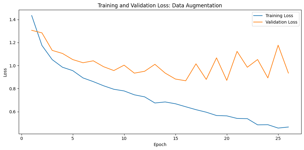
We observe that:
training accuracy is ~.86
validation accuracy is ~.70
plt.rcParams["figure.figsize"] = [10, 5]
plt.rcParams["figure.autolayout"] = True
# accuracy metrics at each iteration are stored in the history variable
acc = history.history['accuracy']
val_acc = history.history['val_accuracy']

loss = history.history['loss']
val_loss = history.history['val_loss']

epochs_range = range(1, len(history.history['loss'])+1)

# Loss
plt.plot(epochs_range, loss, label='Training Loss')
plt.plot(epochs_range, val_loss, label='Validation Loss')
plt.legend(loc='upper right')
plt.title('Training and Validation Loss: Data Augmentation')
plt.xlabel('Epoch')
plt.ylabel('Loss')
plt.show()

# Accuracy
plt.plot(epochs_range, acc, label='Training Accuracy')
plt.plot(epochs_range, val_acc, label='Validation Accuracy')
plt.legend(loc='lower right')
plt.title('Training and Validation Accuracy: Data Augmentation')
plt.xlabel('Epoch')
plt.ylabel('Accuracy')
Text(0, 0.5, 'Accuracy')
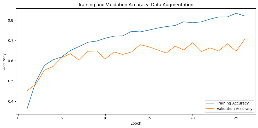
The gap between training and validation performance is smaller!
⚠️ Warning! When doing data augmentation make sure augmented derivatives from the same image do not appear both in your train and validation datasets!
🧑💻 Exercise: Change some of the random transformation parameters and check if there is difference in performance.
🧑💻 Exercise: What other data augmentation techniques can be useful for this problem? Check if they are provided in Keras.
There are other common techniques for overcoming overfitting that it is good to be aware about:
Drop-out: when you apply dropout to a layer, it randomly drops out (by setting the activation to zero) a number of output units from the layer during the training process, which prevents overfitting on specific values (in Keras layers.Dropout)
L1/L2 Regularization: adding an extra penalty term on the weights as in Ridge or Lasso Regression (in Keras regularizers).
Model Testing#
# convert to numpy arrays
test_images, test_labels = zip(*list(test_ds.unbatch()))
test_images = np.array(test_images)
test_labels = np.array(test_labels)
# dense model prediction
dense_model.evaluate(test_images, test_labels)
23/23 ━━━━━━━━━━━━━━━━━━━━ 0s 9ms/step - accuracy: 0.4482 - loss: 1.2866
[1.286587119102478, 0.4482288956642151]
# cnn model prediction
cnn_model.evaluate(test_images, test_labels)
23/23 ━━━━━━━━━━━━━━━━━━━━ 0s 16ms/step - accuracy: 0.6553 - loss: 0.8713
[0.8713046312332153, 0.6553133726119995]
# run only if data augmentation section is run
# cnn_model_aug.evaluate(test_images, test_labels)
# predict with a dense model
dense_pred_labels = dense_model.predict(test_images)
23/23 ━━━━━━━━━━━━━━━━━━━━ 0s 7ms/step
# predict with a CNN model
cnn_pred_labels = cnn_model.predict(test_images)
23/23 ━━━━━━━━━━━━━━━━━━━━ 0s 12ms/step
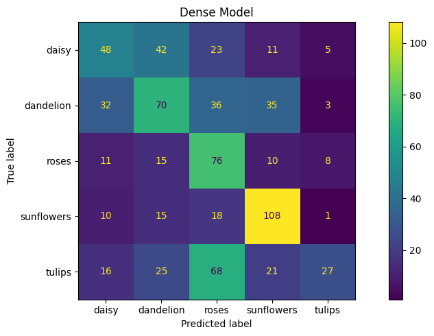
from sklearn.metrics import ConfusionMatrixDisplay
disp = ConfusionMatrixDisplay.from_predictions(test_labels.argmax(axis=1),
                                               dense_pred_labels.argmax(axis=1),
                                               display_labels=class_names,
                                               #normalize='pred',
                                               )
plt.title("Dense Model")
Text(0.5, 1.0, 'Dense Model')
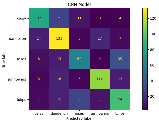
disp = ConfusionMatrixDisplay.from_predictions(test_labels.argmax(axis=1),
                                               cnn_pred_labels.argmax(axis=1),
                                               display_labels=class_names,
                                               #normalize='pred',
                                               )
plt.title("CNN Model")
Text(0.5, 1.0, 'CNN Model')
# display the confusion matrix for the data_augmented model
# ...
Go Out And Collect More Flower Photos!
Recap#
Conceptual Takeaways#
Even simple dense neural networks for relatively small images have a huge number of parameters.
Dense networks require flattening of the image which is not very meaningful for images of different sizes and with objects in different parts of the image. 2D CNNs address these problems.
It is easy to overfit neural network models on small training datasets.
Data augmentation helps building models robust to small variations in the data.
Technical Takeaways#
Neural network libraries have a lot of tools to facilitate the data reading and preprocessing, however, sometimes they are doing steps under the hood that are not obvious.
Identifying when to stop the training may not be trivial when the validation loss and accuracy are noisy.