

Multimodal Models (Notebook)#
Connecting Text and Images with CLIP#
Author: Valentina Staneva

Notebook adapted from CLIP_Intro_Zero_Shot_Classification_and_Embeddings.ipynb by Antonio Rueda-Toicen

Outline#
Read a small dataset of satellite images with matching descriptions from annotators
Load a multimodal CLIP model
Generate image and text embeddings and calculate similarity measures
Demonstrate how to use the model as a zero shot classifier on new descriptions
An Overview of CLIP#
CLIP (Contrastive Language–Image Pre-training) is a model from OpenAI. Given an image and a set of possible text descriptions, the model predicts the most relevant match.
Multimodal Foundation Model. CLIP overcomes traditional challenges in computer vision. One is the reliance on model outputs limited to specific tasks. The model learns to put representations of similar concepts next to each other. It does this regardless whether they are coming from text or images. This happens through extensive training with text-image pairs scraped from the internet.
Zero-shot Classification. CLIP adapts to new visual classification tasks without changes in the model’s architecture. This is zero-shot inference. It differs from standard image classification models. Those only predict the predefined classes that they were trained on.
Contrastive pre-training#

Encoders
Image encoder: either a Vision Transformer or a CNN Resnet.
Text Encoder: BERT-like transformer or a Continuous Bag of Words (CBOW)
Encode inputs into a “joint” space: similar concepts in text and images
Contrastive Loss. Given \(N\) images and their \(N\) matching descriptions, CLIP is trained to predict which of the \(NXN\) matchings of image pairs occurred. We jointly train an image encoder and a text encoder to maximize cosine similarity of the matching \(N\) pairs (main diagonal on the plot), while minimizing similarity of tne \(N ^ 2 - N\) incorrect pairings. The cross entropy of images to text and the cross entropy of text to images is added and averaged. This is called ‘symmetric cross entropy’ and is the ‘contrastive loss’ used to train the model. The pseudocde of the method, from the original paper by OpenAI, is shown below.

With this method, embeddings that represent similar concepts are moved closer together. The effect is what we see in the image below. Embeddings of text and images with high semantic similarity get close to each other. Semantically different text-image pairs are kept further apart.
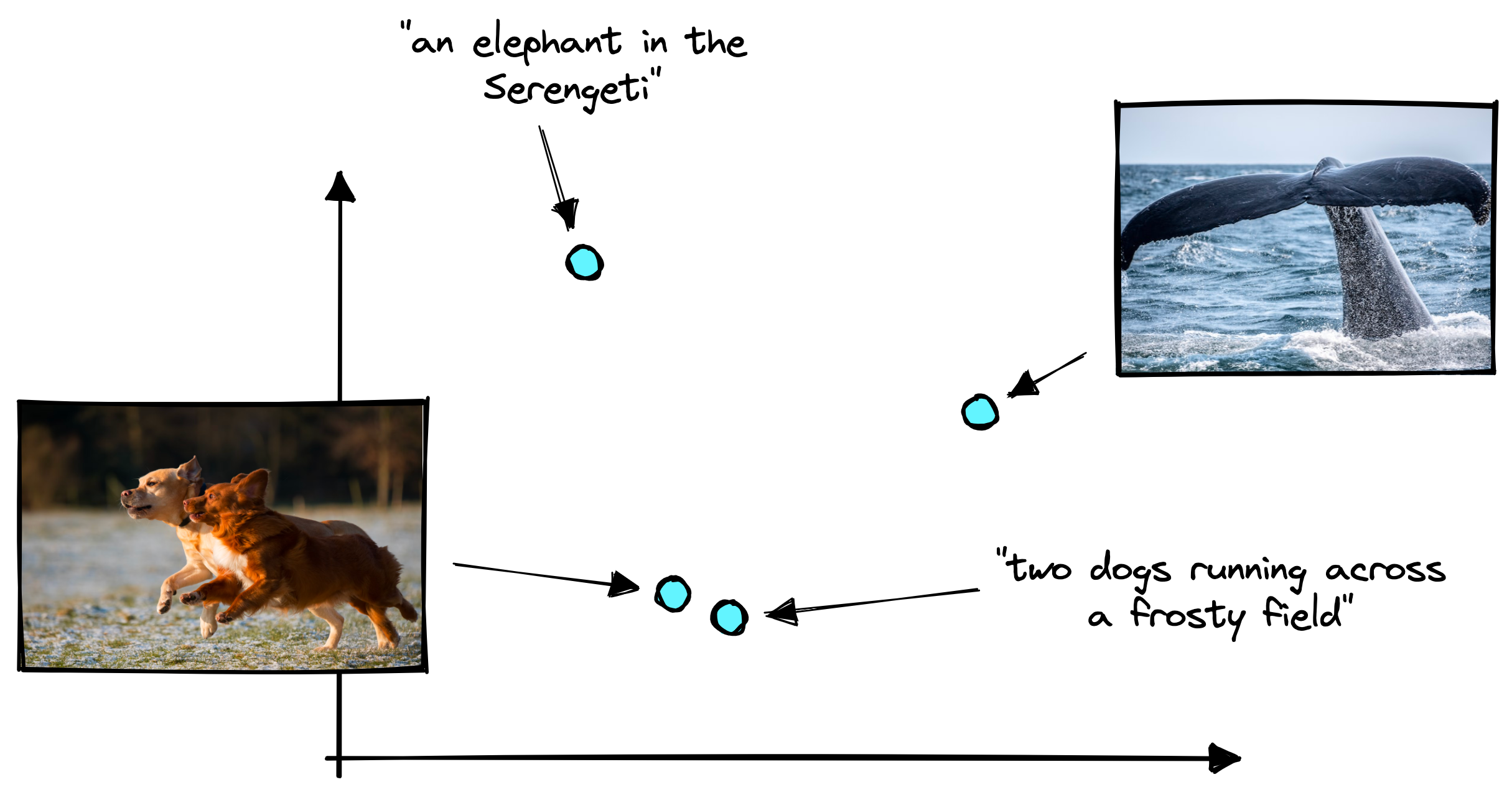
In this notebook, we use CLIP to extract image embeddings. We don’t delve further into contrastive pre-training, which takes substantial computational resources.
Zero-shot image classification#
CLIP can be applied to any visual classification benchmark. We do this by providing the names of the visual categories to classify. Zero-shot prediction allows us generalize on unseen labels. We don’t need to specifically train the model to classify them. For example, all ImageNet pretrained models recognize 1000 specific classes. CLIP is not bound by this limitation. With CLIP, we can create new labels ‘on the fly’. We pass them through the text encoder. Then we use the similarity between text and image embeddings to produce an output.

Limitations and issues#
Generalization beyond training data. CLIP has its limitations. It has difficulty with abstract tasks. It’s also difficult to generalize to images outside the pre-training dataset. We sometimes need to finetune the model to do good fine-grained classification.
Ethical concerns regarding data collection. Ethical concerns arise due to the potential for biases coming from the dataset. There are also privacy and copyright issues. A lot of data from the Internet was used to train this model. Despite these challenges, CLIP’s ability highlights the usefulness of applying Internet-scale multimodal datasets.
Computational challenges. The original CLIP model was trained on 400 million image-text pairs. This was done using 256 V100 Nvidia GPUs. This scale is unachievable by most companies and private individuals. It’s difficult to create a CLIP model from scratch that performs as well as the pretrained ones by OpenAI or LAION.
In this notebook we will explore both the capabilities and limitations of CLIP.
# uncomment to download the dataset
#!gdown --id 1L4lBSL0SIVP2t24TbZEBTBerroGBC7p-
# uncomment to unzip the dataset
#!unzip satellite-image-captioning.zip
Reading Data#
import pandas as pd
labels = pd.read_csv('satellite-image-captioning/train.csv')
import skimage.io as sk_io
from PIL import Image
from collections import OrderedDict
def get_image_and_description(filename):
  # get only the first description
  description = labels[labels['filepath']==filename]['captions'].iloc[0].split('\n')[0].strip("['").strip('"')
  img = Image.fromarray(sk_io.imread(f'satellite-image-captioning/{filename}'))
  return img, description
sample_files = ['train/industrial_120.jpg','train/desert_123.jpg', 'train/mountain_116.jpg', 'train/beach_261.jpg', 'train/forest_40.jpg', 'train/pond_100.jpg', 'train/farmland_349.jpg' ]
imgs, descriptions = zip(*[get_image_and_description(filename) for filename in sample_files])
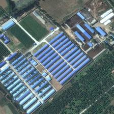
print(descriptions[0])
imgs[0]
Many green buildings and trees are located in an industrial area.
Loading a pretrained CLIP model#
from transformers import CLIPModel, CLIPProcessor
import torch
from PIL import Image
import requests
# We have downloaded both the architecture and the model's weights.
model = CLIPModel.from_pretrained('openai/clip-vit-base-patch32')
# model
CLIPModel.from_pretrained('openai/clip-vit-base-patch32') is a function call that loads a pre-trained CLIP model, the clip-vit-base-patch32 version.
Here’s what happens during this function call:
Model Architecture Loading: The
CLIPModelclass represents the CLIP model architecture. When we callfrom_pretrained(), it initializes a model with the architecture defined for CLIP.Pre-trained Weights: The string
'openai/clip-vit-base-patch32'is a set of weights. These weights are in the Hugging Face model hub. OpenAI produced these with the CLIP learning method on a large dataset of images and their descriptions.Vision Transformer Variant:
vit-base-patch32indicates that the model uses the Vision Transformer (ViT) architecture. The input images are divided into patches of size 32x32 pixels before processing by the transformer. We could also choose a ResNet (convolutional neural network) instead.Downloading and Caching: If this is the first time we’re using this model in the running working space, the weights are downloaded from the Hugging Face model hub and cached locally. The following usage of
from_pretrained()will use the local cache, without downloading the weights again.Instantiation and Readiness for Inference: After the model weights load, the CLIP model is ready for inference. You can then process images and text to extract text of image features (vector embeddings) or perform zero-shot classification tasks.
processor = CLIPProcessor.from_pretrained('openai/clip-vit-base-patch32')
processor
CLIPProcessor:
- image_processor: CLIPImageProcessor {
  "crop_size": {
    "height": 224,
    "width": 224
  },
  "do_center_crop": true,
  "do_convert_rgb": true,
  "do_normalize": true,
  "do_rescale": true,
  "do_resize": true,
  "image_mean": [
    0.48145466,
    0.4578275,
    0.40821073
  ],
  "image_processor_type": "CLIPImageProcessor",
  "image_std": [
    0.26862954,
    0.26130258,
    0.27577711
  ],
  "resample": 3,
  "rescale_factor": 0.00392156862745098,
  "size": {
    "shortest_edge": 224
  }
}

- tokenizer: CLIPTokenizer(name_or_path='openai/clip-vit-base-patch32', vocab_size=49408, model_max_length=77, padding_side='right', truncation_side='right', special_tokens={'bos_token': '<|startoftext|>', 'eos_token': '<|endoftext|>', 'unk_token': '<|endoftext|>', 'pad_token': '<|endoftext|>'}, added_tokens_decoder={
	49406: AddedToken("<|startoftext|>", rstrip=False, lstrip=False, single_word=False, normalized=True, special=True),
	49407: AddedToken("<|endoftext|>", rstrip=False, lstrip=False, single_word=False, normalized=False, special=True),
})

{
  "image_processor": {
    "crop_size": {
      "height": 224,
      "width": 224
    },
    "do_center_crop": true,
    "do_convert_rgb": true,
    "do_normalize": true,
    "do_rescale": true,
    "do_resize": true,
    "image_mean": [
      0.48145466,
      0.4578275,
      0.40821073
    ],
    "image_processor_type": "CLIPImageProcessor",
    "image_std": [
      0.26862954,
      0.26130258,
      0.27577711
    ],
    "resample": 3,
    "rescale_factor": 0.00392156862745098,
    "size": {
      "shortest_edge": 224
    }
  },
  "processor_class": "CLIPProcessor"
}
The CLIPProcessor prepares data for CLIP. The model requires both images and text to be in a specific format before being fed to the encoding networks. Here’s how it works:
Resizing and Normalization: The processor takes an image input. It then resizes it to the dimensions expected by the model (e.g., 224x224 pixels). It then normalizes the image by scaling pixel values to a range that the model was trained on, typically [0, 1] or [-1, 1]. It then aligns it with the color channel means and standard deviations that the model expects. For this model these are the mean and standard deviations of the RGB channels on the CLIP training dataset. CLIP was trained from scratch by OpenAI without using ImageNet weights for the visual encoder or other weights for the text encoder.
Tokenization: For the text inputs, the processor tokenizes the sentences. We convert the text to tokens (often words or syllables) that are represented by numerical IDs. These IDs correspond to entries in the model’s vocabulary.
Padding and Attention Mask: The processor pads the token sequences. They are made to be the same length for batch processing. It also creates attention masks that allow the model to ignore padding tokens during processing.
Conversion to PyTorch Tensors: The processor converts the processed image and text data into PyTorch tensors. Tensors are multi-dimensional arrays suitable for input into the model.
Return Tensors: The processed tensors return in a format that can be fed into the CLIP model. Now we can produce classifications or embeddings from them.
Text Embeddings#
inputs = processor(text=descriptions, return_tensors="pt",
                   padding=True, truncation=True)

# We use torch.no_grad() to avoid having to call .detach() on the tensor
with torch.no_grad():
    text_embeddings = model.get_text_features(**inputs)
# the final output dimension
text_embeddings.pooler_output[0].shape
torch.Size([512])
Image Embeddings#
inputs = processor(images=imgs,
                   return_tensors="pt")
📝 Note: The images are normalized based on the mean and std of the training set which can result in values outside of the range between -1 and 1.
print(inputs['pixel_values'].min(), inputs['pixel_values'].max())
tensor(-1.7923) tensor(2.1459)
image_embeddings = model.get_image_features(**inputs)
# the final output dimension
image_embeddings.pooler_output[0].shape
torch.Size([512])
📝 Note The double asterisk ** is used to unpack the inputs dictionary into keyword arguments. This means that if inputs contains, {'pixel_values':tensor, 'attention_mask': tensor}, calling **inputs would be like passing pixel_values=tensor, attention_mask=tensor directly to the function.
Cosine Similarity#
torch.nn.CosineSimilarity
dim: This parameter specifies the dimension along which cosine similarity is computed.dim=0means that the similarity will be computed along the first dimension (i.e., the rows if we think of a 2D tensor as a matrix).eps: This is a small value added to the denominator for numerical stability. In the code eps=1e-6, it prevents division by zero when normalizing vectors. This is especially useful when dealing with very small values in the vectors.
cosine_similarity = torch.nn.CosineSimilarity(dim=0, eps=1e-6)
def show_pair(imag_a, imag_b):
  plt.subplot(121)
  plt.imshow(np.array(imag_a))
  plt.axis("off")

  plt.subplot(122)
  plt.imshow(np.array(imag_b))
  plt.axis("off")
Evaluating the similarity of image embeddings#
import matplotlib.pyplot as plt
import numpy as np
# @title {run:'auto'}

slider_value_1 = 0  # @param {type: "slider", min: 0, max: 6}
slider_value_2 = 6  # @param {type: "slider", min: 0, max: 6}


# Access the pooler_output attribute for the image embeddings to get the 512-dimensional features
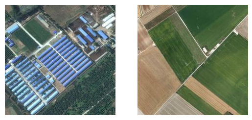
print(f'Cosine similarity = {cosine_similarity(image_embeddings.pooler_output[slider_value_1], image_embeddings.pooler_output[slider_value_2]):.2f}')
show_pair(imgs[slider_value_1], imgs[slider_value_2])
Cosine similarity = 0.72
Evaluating the similarity of text embeddings#
# @title {run:'auto'}

slider_value_1 = 0  # @param {type: "slider", min: 0, max: 6}
slider_value_2 = 6  # @param {type: "slider", min: 0, max: 6}


print(f"""Cosine similarity = {cosine_similarity(text_embeddings.pooler_output[slider_value_1],
                                               text_embeddings.pooler_output[slider_value_2]):.2f}""")
print(f"""First description: {descriptions[slider_value_1]}\nSecond description: {descriptions[slider_value_2]}""")
Cosine similarity = 0.83
First description: Many green buildings and trees are located in an industrial area.
Second description: the green fields are surrounded by bare land.
Evaluating the text-image similarity of embeddings#
# @title {run:'auto'}

slider_value_1 = 0  # @param {type: "slider", min: 0, max: 6}
slider_value_2 = 0  # @param {type: "slider", min: 0, max: 6}


print(f"""Cosine similarity = {cosine_similarity(text_embeddings.pooler_output[slider_value_1],
                                                image_embeddings.pooler_output[slider_value_2]):.2f}""")
print(f"""Description: {descriptions[slider_value_1]}""")
imgs[slider_value_2]
Cosine similarity = 0.27
Description: Many green buildings and trees are located in an industrial area.
# Notice that the embeddings are not normalized
text_embeddings.pooler_output.max(), image_embeddings.pooler_output.max()
(tensor(5.9163), tensor(3.0462, grad_fn=<MaxBackward1>))
# We normalize embeddings (the cosine_similarity function did this for us before)
image_embeddings.pooler_output /= image_embeddings.pooler_output.norm(dim=-1, keepdim=True)
text_embeddings.pooler_output /= text_embeddings.pooler_output.norm(dim=-1, keepdim=True)
text_embeddings.pooler_output.max(), image_embeddings.pooler_output.max()
(tensor(0.5729), tensor(0.3109, grad_fn=<MaxBackward1>))
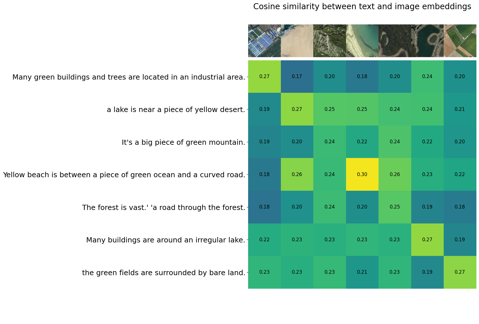
similarity = text_embeddings.pooler_output @ image_embeddings.pooler_output.T
similarity
tensor([[0.2686, 0.1731, 0.1978, 0.1808, 0.1992, 0.2379, 0.2004],
        [0.1948, 0.2663, 0.2474, 0.2462, 0.2405, 0.2391, 0.2064],
        [0.1900, 0.1982, 0.2361, 0.2203, 0.2443, 0.2215, 0.2043],
        [0.1809, 0.2634, 0.2354, 0.2962, 0.2551, 0.2260, 0.2176],
        [0.1760, 0.2014, 0.2373, 0.1995, 0.2482, 0.1893, 0.1834],
        [0.2239, 0.2296, 0.2268, 0.2319, 0.2279, 0.2674, 0.1921],
        [0.2315, 0.2264, 0.2344, 0.2056, 0.2317, 0.1939, 0.2652]],
       grad_fn=<MmBackward0>)
count = len(descriptions)

plt.figure(figsize=(20, 14))
plt.imshow(similarity.detach(), vmin=0.1, vmax=0.3)
plt.yticks(range(count), descriptions, fontsize=18)
plt.xticks([])
for i, image in enumerate(imgs):
    plt.imshow(image, extent=(i - 0.5, i + 0.5, -1.6, -0.6), origin="lower")
for x in range(similarity.shape[1]):
    for y in range(similarity.shape[0]):
        plt.text(x, y, f"{similarity[y, x]:.2f}", ha="center", va="center", size=12)

for side in ["left", "top", "right", "bottom"]:
  plt.gca().spines[side].set_visible(False)

plt.xlim([-0.5, count - 0.5])
plt.ylim([count + 0.5, -2])

plt.title("Cosine similarity between text and image embeddings", size=20);
Running CLIP as a zero-shot classifier#
text = ['blue long buildings',
        'buildings',
        'sand with a little water',
        'planted trees',
        'forest',
        'park',
        'plant',
        'parking lot',
        # 'parking lot with trucks'
        #'field',
        #'satellite image'
        ]

inputs = processor(text=text,
                   images=imgs,
                   return_tensors="pt", padding=True)
outputs = model(**inputs)
probs = outputs.logits_per_image.softmax(dim=1)
# @title Probabilities per description {run:'auto'}

slider_value = 0  # @param {type: "slider", min: 0, max: 7}

# Creating a subplot with an image in the first row and the histogram in the second row
fig, axes = plt.subplots(1, 2, figsize=(12, 5))

axes[1].imshow(np.array(imgs[slider_value]))
axes[1].axis('off')  # Turning off the axis for the image
axes[1].set_title(descriptions[slider_value])

probs = outputs.logits_per_image.softmax(dim=1)

# Creating the horizontal bar plot in the second subplot
axes[0].barh(text, probs[slider_value].detach(), color='skyblue')
axes[0].set_xlim(0, 1)  # Setting the x-axis limit from 0 to 1

axes[0].set_xlabel('Probabilities')
axes[0].set_title('Probabilities of Labels')

plt.tight_layout()
plt.show()
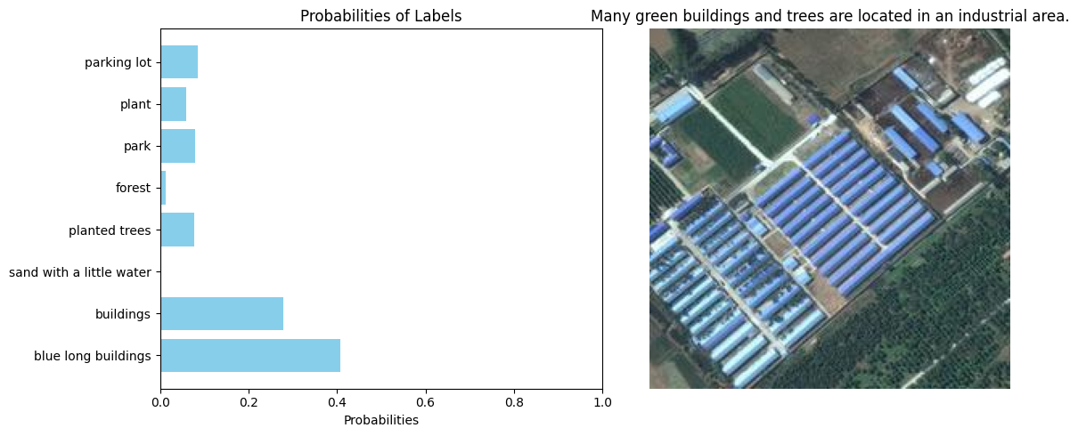
🧑💻 Exercise: Try adding some descriptions (matching or not matching) on your own. Change the image by moving the slider.
Description Specificity#
Check out the probabilities that our zero shot classifier outputs when we make the description of the image more specific.
# Notice what happens with the output probabilities
# when we make the labels more specific
text = ['buldings',
        'long buildings',
        'long buildings and planted trees',
        'a satellite image of long buildings and planted trees',
        # add your description
        ]

inputs = processor(text=text,
                   images=[imgs[0]],
                   return_tensors="pt", padding=True)
outputs = model(**inputs)
logits_per_image = outputs.logits_per_image
# Creating a subplot with an image in the first row and the histogram in the second row
fig, axes = plt.subplots(1, 2, figsize=(12, 5))

axes[1].imshow(np.array(imgs[0]))
axes[1].axis('off')  # Turning off the axis for the image

probs = (logits_per_image).softmax(dim=1)

# Creating the horizontal bar plot in the second subplot
axes[0].barh(text, probs.detach().numpy().flatten(), color='skyblue')
axes[0].set_xlim(0, 1)  # Setting the x-axis limit from 0 to 1

axes[0].set_xlabel('Probabilities')
axes[0].set_title('Probabilities of Different Labels')

plt.tight_layout()
plt.show()
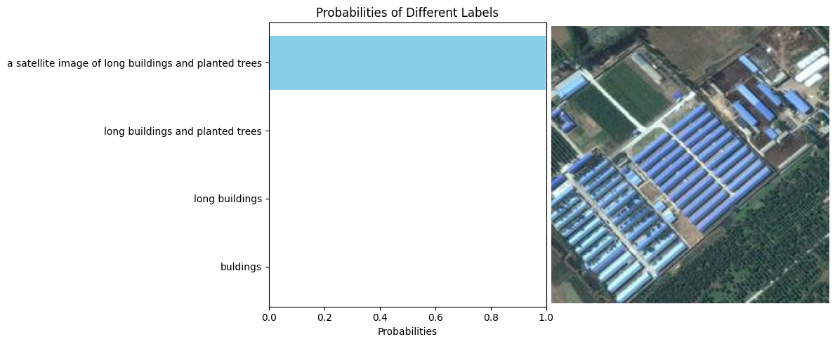
🧑💻 Exercise: Add a more specific description, or a more general one. Change the image by passing a different index to imgs.
🧑💻 Exercise: We only used a few images, but the folder has many files. Can you set up a system to query the images by providing a text description.
Recap#
Conceptual Takeaways#
By generating text and image embeddings we can compute similarities not only between images, and between texts, but also between texts and images.
The contrastive loss in the CLIP model allows us to match best possible image or text to a sample, without having to have exact same categories.
Technical Takeaways#
The similarity scores may not be that different for the same type of images and descriptions coming from the same dataset.
While the hidden dimensions of the image and text embeddings are different the
pooler_outputbrings them to the same dimension.