W   UNIVERSITY of WASHINGTON  ·  eScience Institute
AI IN PRACTICE WORKSHOP

Sequence Models

What you do here

Section	What happens	Why it matters
0	Setup	Imports and the weather dataset
1	Sequence data and its shapes	What makes data a sequence, and the four shapes of sequence problems
2	Meet the data	Eight years of hourly temperature, the signal we forecast
3	Frame the forecast	Slice one long series into (window, target) training examples
4	The naive baseline	The trivial number every real model has to beat
5	A training helper	One function, so the focus stays on the architecture
6	A ladder of models	Dense, 1-D CNN, RNN, LSTM, each fixing the weakness before it
7	Compare the models	Same data, same metric, an honest comparison
8	See the predictions	Where a model tracks the signal, and where it misses
9	Your turn	Bidirectional, stacked, and window-size experiments
10	Takeaways	What carries into tomorrow

Frameworks. Everything today uses Keras (TensorFlow), the same stack as this morning.

Before you start. A GPU is not required: the models are small and train in seconds to a couple of minutes on CPU. Run the two setup cells below first, to import the libraries and download the dataset.

0 - Setup (run this first)

Run the two cells below first: they import the libraries and download the dataset.

# Standard scientific stack, all preinstalled on Colab.
import numpy as np
import matplotlib.pyplot as plt
import tensorflow as tf
from tensorflow import keras
from tensorflow.keras import layers

# Reproducibility
keras.utils.set_random_seed(42)

# UW-purple styling for our plots
UW_PURPLE, UW_GOLD, UW_PINK = "#4B2E83", "#85754D", "#C42A8B"
plt.rcParams.update({"axes.edgecolor": "#6B6580", "axes.labelcolor": "#221C35",
                     "figure.facecolor": "white", "axes.grid": True,
                     "grid.color": "#E5E0EE", "grid.linewidth": 0.8})

print("TensorFlow:", tf.__version__)
print("GPU available:", "YES" if tf.config.list_physical_devices('GPU') else "no (CPU is fine for today)")

TensorFlow: 2.20.0
GPU available: YES

# Download the Jena Climate dataset (weather near Jena, Germany; 2009–2016,
# recorded every 10 minutes). ~13 MB, cached after the first run.
import os
from zipfile import ZipFile

zip_path = keras.utils.get_file(
    "jena_climate_2009_2016.csv.zip",
    "https://storage.googleapis.com/tensorflow/tf-keras-datasets/jena_climate_2009_2016.csv.zip",
)
csv_dir = os.path.dirname(zip_path)
csv_path = os.path.join(csv_dir, "jena_climate_2009_2016.csv")
if not os.path.exists(csv_path):
    with ZipFile(zip_path) as z:
        z.extractall(csv_dir)
print("CSV ready at:", csv_path)

Downloading data from https://storage.googleapis.com/tensorflow/tf-keras-datasets/jena_climate_2009_2016.csv.zip
13568290/13568290 ━━━━━━━━━━━━━━━━━━━━ 2s 0us/step
CSV ready at: /root/.keras/datasets/jena_climate_2009_2016.csv

1 - Sequence data, and the shapes of sequence problems

This morning you worked with fixed-size inputs: an image is always the same grid of pixels, available to the model all at once. A sequence is different. It is an ordered list of values, x_1, x_2, …, x_T, with three defining properties:

• Order carries meaning. Swapping two elements can change the meaning entirely. “The dog bit the man” and “The man bit the dog” use the same words but describe different events.

• Length can vary. A sentence can be five words or fifty; a weather record can span a day or a decade.

• Nearby elements tend to be related. Today’s temperature is a strong clue about tomorrow’s; the previous word constrains which word is likely to come next.

Sequential data is everywhere: text (a sequence of words), audio (amplitude samples), DNA (nucleotides), sensor logs, stock prices, and, in our case today, hourly temperature readings.

The shapes of sequence problems

Not every sequence problem has the same form. They differ in how many steps go in and how many come out, and that shape decides which model and which kind of output make sense:

• many-to-one: a whole window of inputs collapses to a single output. Classifying a review as positive or negative, or forecasting one future value from a window of past ones.

• one-to-many: a single input expands into a sequence. Generating a caption from one image.

• many-to-many (aligned): one output per input step, in lockstep. Tagging every word in a sentence with its part of speech.

• seq2seq (many-to-many, unaligned): an input sequence maps to an output sequence of a different length. Translating a sentence between languages.

Red boxes are inputs, green boxes are the RNN carrying its hidden state forward, and blue boxes are outputs. Reading left to right: a plain network with no sequence at all, then the four shapes above, in the same order as the bullets.

Source: Andrej Karpathy, “The Unreasonable Effectiveness of Recurrent Neural Networks,” karpathy.github.io, 2015. karpathy.github.io/2015/05/21/rnn-effectiveness

Which shape is your research problem? Before building anything, map your own data onto one of these:

Your data looks like…	…then reach for
one label for a whole window	many-to-one
a sequence generated from a seed	one-to-many
a label for every timestep	many-to-many (aligned)
one sequence mapped to another	seq2seq (tomorrow’s transformers shine here)

Today we take the first shape, many-to-one, and follow it from start to finish: we feed a window of past hourly temperatures (many steps in) and predict a single temperature 24 hours ahead (one out). Everything below, framing the data, building a baseline, and climbing a ladder of models, is that one shape made concrete. Keep the table in mind and think about which row your own problem fits.

2 - Meet the data: hourly temperature

To make many-to-one forecasting concrete we use a real signal: eight years of weather recorded near Jena, Germany, sampled every ten minutes. We load it, resample to hourly readings to keep training fast, and look at it before framing the forecast.

# Read the CSV with plain numpy (no pandas needed).
raw = np.genfromtxt(csv_path, delimiter=",", skip_header=1,
                    usecols=range(1, 15), invalid_raise=False)
header = open(csv_path).readline().strip().split(",")
col_names = [c.strip('"') for c in header[1:15]]
print("Columns:", col_names)

# Temperature is the "T (degC)" column
TEMP_COL = col_names.index("T (degC)")
temperature = raw[:, TEMP_COL].astype("float32")
print("Total 10-minute readings:", len(temperature))

Columns: ['p (mbar)', 'T (degC)', 'Tpot (K)', 'Tdew (degC)', 'rh (%)', 'VPmax (mbar)', 'VPact (mbar)', 'VPdef (mbar)', 'sh (g/kg)', 'H2OC (mmol/mol)', 'rho (g/m**3)', 'wv (m/s)', 'max. wv (m/s)', 'wd (deg)']
Total 10-minute readings: 420551

# 10-minute data is dense and slow to train on. Resample to HOURLY (every 6th row).
temp = temperature[::6]
print("Hourly readings:", len(temp))

fig, ax = plt.subplots(1, 2, figsize=(13, 3.5))
ax[0].plot(temp[:24*10], color=UW_PURPLE)
ax[0].set_title("First 10 days (hourly)"); ax[0].set_xlabel("hour"); ax[0].set_ylabel("°C")
ax[1].plot(temp, color="#1FA39B", lw=0.5)
ax[1].set_title("All 8 years"); ax[1].set_xlabel("hour"); ax[1].set_ylabel("°C")
plt.tight_layout(); plt.show()

Hourly readings: 70092

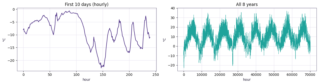
Discuss: notice the daily cycle in the 10-day plot and the yearly cycle in the 8-year plot. Both are signals a forecasting model can exploit: today’s temperature is correlated with yesterday’s (the daily cycle) and with the temperature around the same time last year (the yearly cycle). A good model uses the recent past to anticipate the near future. That is our task below.

3 - Frame the forecast: windowing

Neural networks are trained with supervised learning: pairs of (input, target). A raw temperature series is just one long sequence of numbers, with no obvious inputs or targets, so before training anything we need to turn it into a supervised learning problem.

The standard technique is a sliding window: cut a fixed-length stretch of the past (the input) and pair it with a single value some fixed distance later (the target). Sliding this window forward one step at a time turns one long series into thousands of overlapping (input window -> future target) examples. Getting this framing right matters more than any model choice that follows: get it wrong, for example by letting future values leak into the input, and every model built on top of it will look artificially good or bad.

• Input: the last SEQ_LEN hours of temperature. Target: the temperature DELAY hours after the window ends.

• SEQ_LEN controls how much history the model can see (its receptive field in time); DELAY controls how far ahead we are forecasting (the forecast horizon).

# --- Problem settings ---------------------------------------------------
SEQ_LEN  = 48     # look back 48 hours (2 days)
DELAY    = 24     # predict the temperature 24 hours ahead
BATCH    = 128

FAST_DEMO = False  # ← keeps the live session snappy. Set False for full data / better numbers.
if FAST_DEMO:
    temp_use = temp[:25000]    # ~3 years, trains in seconds–minutes
    EPOCHS   = 10
else:
    temp_use = temp
    EPOCHS   = 25

# Chronological split: train on the PAST, validate/test on the FUTURE (never shuffle across time!)
n   = len(temp_use)
ntr = int(n * 0.6)
nva = int(n * 0.2)
print(f"train {ntr} | val {nva} | test {n-ntr-nva} hours")

train 15000 | val 5000 | test 5000 hours

# Normalize using TRAIN statistics only (don't peek at val/test).
mu = temp_use[:ntr].mean()
sd = temp_use[:ntr].std()
norm = ((temp_use - mu) / sd).astype("float32").reshape(-1, 1)   # shape (n, 1): one feature
print(f"train mean={mu:.2f}°C  std={sd:.2f}°C")

train mean=9.00°C  std=8.99°C

Keras provides a utility, timeseries_dataset_from_array, that implements exactly this sliding-window slicing for us, so we do not have to write the indexing logic by hand.

def make_dataset(arr, start, end, shuffle):
    inputs  = arr[start : end - DELAY]
    targets = arr[start + SEQ_LEN + DELAY - 1 : end, 0]
    return keras.utils.timeseries_dataset_from_array(
        inputs, targets, sequence_length=SEQ_LEN, batch_size=BATCH, shuffle=shuffle)

train_ds = make_dataset(norm, 0,        ntr,      shuffle=True)
val_ds   = make_dataset(norm, ntr,      ntr+nva,  shuffle=False)
test_ds  = make_dataset(norm, ntr+nva,  n,        shuffle=False)

for x, y in train_ds.take(1):
    print("input batch :", x.shape, "  <- (batch, SEQ_LEN, 1 feature)")
    print("target batch:", y.shape)
N_FEAT = x.shape[-1]

input batch : (128, 48, 1)   <- (batch, SEQ_LEN, 1 feature)
target batch: (128,)

See it concretely. The cell below prints two consecutive windows from the real data, so you can watch the window slide by one step: the same idea as the diagram above, now with actual numbers.

xb, yb = next(iter(val_ds))          # val_ds is unshuffled, so samples are consecutive
print("window 0 (first 6 hrs, normalized):", np.round(xb[0, :6, 0].numpy(), 2), "...")
print("window 1 (first 6 hrs, normalized):", np.round(xb[1, :6, 0].numpy(), 2), "...  ← slid by one step")
print()
print(f"their targets in °C: {yb[0]*sd+mu:.1f}  and  {yb[1]*sd+mu:.1f}")

window 0 (first 6 hrs, normalized): [0.19 0.14 0.13 0.13 0.12 0.13] ...
window 1 (first 6 hrs, normalized): [0.14 0.13 0.13 0.12 0.13 0.12] ...  ← slid by one step

their targets in °C: 6.8  and  6.4

4 - The naive baseline and MAE

Before training any neural network, we need a baseline: a simple rule that any real model must beat to be worth using. In forecasting, the standard baseline is persistence: predict that the future value equals the most recent observed value (“tomorrow’s temperature is about the same as right now”). Persistence works surprisingly well for smooth, slowly changing signals like temperature, which is exactly why it makes a fair and demanding baseline.

We measure error with Mean Absolute Error (MAE):

MAE = average of |prediction - actual| over all examples.

MAE is reported in the same units as the target (degrees Celsius here), so an MAE of 2.0 means the model is, on average, off by about 2 degrees. That makes it much easier to interpret than a squared-error metric.

def naive_mae(ds):
    errs = []
    for x, y in ds:
        # TODO: the naive prediction is the LAST value in each window.
        #       x has shape (batch, SEQ_LEN, 1). Grab the last timestep.
        last_value = x[:,-1, 0]                          # <-- fill this in
        errs.append(tf.reduce_mean(tf.abs(last_value - y)))
    return float(tf.reduce_mean(errs)) * sd

baseline_mae = naive_mae(val_ds)
print(f"Naive baseline MAE: {baseline_mae:.2f} °C")

Naive baseline MAE: 2.82 °C

Hint

last_value = x[:, -1, 0]

5 - A training helper

Every model below will be compiled, trained, and evaluated the same way. Rather than repeat that boilerplate five times, we wrap it in one helper function so the rest of the notebook can focus on what actually changes between models: the architecture.

results = {"naive": baseline_mae}        # collect every model's MAE here

early = keras.callbacks.EarlyStopping(patience=3, restore_best_weights=True)

def train_and_score(model, name):
    model.compile(optimizer="adam", loss="mse", metrics=["mae"])
    hist = model.fit(train_ds, validation_data=val_ds,
                     epochs=EPOCHS, callbacks=[early], verbose=0, shuffle=False)
    mae_C = model.evaluate(val_ds, verbose=0)[1] * sd
    results[name] = mae_C
    print(f"{name:>10s}  val MAE = {mae_C:5.2f} °C   "
          f"({'beats' if mae_C < baseline_mae else 'loses to'} naive {baseline_mae:.2f})")
    return hist

6 - A ladder of models

We will train five models on the same data with the same evaluation metric. Each one is a small change from the last, and each change fixes a specific weakness of the model before it. Keep the table below in view as a map for what follows:

6a - Dense network: ignores order

A fully connected (dense) layer takes a fixed-size vector and learns a weighted combination of its entries. To use one here, we first Flatten the window from shape (SEQ_LEN, N_FEAT) into a single vector of SEQ_LEN * N_FEAT numbers.

This works, in the sense that the network can still learn a useful mapping. But flattening discards the window’s structure: position 1 and position 48 become two entries in a list, with nothing telling the model that one came before the other, or how far apart they are. The model has to learn any temporal structure from scratch, and the number of parameters grows with the window length.

dense = keras.Sequential([
    keras.Input(shape=(SEQ_LEN, N_FEAT)),
    layers.Flatten(),
    # TODO: add one Dense hidden layer (32 units, relu) and a Dense(1) output
    layers.Dense(32, activation = "relu"),
    layers.Dense(1),

])
train_and_score(dense, "dense")

     dense  val MAE =  2.77 °C   (beats naive 2.82)

<keras.src.callbacks.history.History at 0x7a41f8ffa1e0>

Hint

layers.Dense(32, activation="relu"),
layers.Dense(1),

6b - 1-D convolution: local patterns

A 1-D convolution applies the same small filter (a short vector of learned weights) at every position along the sequence, computing a weighted sum over a short window as it slides. Because the same filter is reused everywhere, the network learns to detect a local pattern, such as a sudden spike or dip, wherever it occurs, using far fewer parameters than a dense layer would need for the same job. This weight sharing is the same idea a 2-D CNN uses on images, applied along a single time axis instead of two spatial axes.

The tradeoff is the filter’s field of view: a kernel of size 5 can only look at 5 consecutive timesteps at once. Stacking more convolution layers widens that view, but a 1-D CNN on its own has no built-in way to combine information across the whole window, which is what the next model adds.

cnn = keras.Sequential([
    keras.Input(shape=(SEQ_LEN, N_FEAT)),
    # TODO: a Conv1D (32 filters, kernel_size=5, relu),
    #       then GlobalAveragePooling1D(), then Dense(1)
    layers.Conv1D(32, kernel_size = 5, activation = "relu"),
    layers.GlobalAveragePooling1D(),
    layers.Dense(1),
])
train_and_score(cnn, "cnn")

       cnn  val MAE =  3.89 °C   (loses to naive 2.82)

<keras.src.callbacks.history.History at 0x7a41f91104d0>

Hint

layers.Conv1D(32, kernel_size=5, activation="relu"),
layers.GlobalAveragePooling1D(),
layers.Dense(1),

6c - SimpleRNN: memory across steps

A recurrent neural network (RNN) processes a sequence one timestep at a time, in order. At each step it combines the current input with a hidden state (a vector summarizing everything seen so far) to produce a new hidden state:

h_t = tanh(W_x * x_t + W_h * h_(t-1) + b)

The important part is that the same cell, and the same weights W_x, W_h, b, are reused at every timestep. This is weight sharing again, now applied along time instead of across an image. Unrolling the loop into a chain (right side of the diagram below) makes this concrete: it is the identical small network, applied repeatedly.

The hidden state is best understood as a running summary: at every step, new summary = combine(old summary, new input). The circle below “fills up” as context accumulates:

Because the hidden state is a fixed-size vector that gets overwritten at every step, its capacity is limited: information from many steps ago has to survive being repeatedly combined with newer inputs, and in practice it tends to fade. That fading is the weakness the next model is built to fix.

rnn = keras.Sequential([
    keras.Input(shape=(SEQ_LEN, N_FEAT)),
    # TODO: a SimpleRNN with 32 units, then Dense(1)
    layers.SimpleRNN(32),
    layers.Dense(1)
])
train_and_score(rnn, "rnn")

       rnn  val MAE =  2.78 °C   (beats naive 2.82)

<keras.src.callbacks.history.History at 0x7a429664ad20>

Hint

layers.SimpleRNN(32),
layers.Dense(1),

6d - LSTM: protected long memory

Before fixing the problem, it helps to see it stated plainly. During training, the error signal has to travel backward through every timestep the network processed, a process called backpropagation through time. At each step backward, the signal is multiplied by a small number, so after many steps it shrinks toward zero: a well-known issue called the vanishing gradient. In practice this means a plain RNN’s weights barely update in response to something that happened far in the past, so long-range dependencies (like a subject and a verb separated by many words) get lost.

The same idea, in its classic form: the earlier the relevant input (highlighted in red below), the harder it is for that information to influence a distant output.

Source: Christopher Olah, “Understanding LSTM Networks,” colah’s blog, 2015. colah.github.io/posts/2015-08-Understanding-LSTMs

A Long Short-Term Memory (LSTM) cell fixes this by adding a second, protected pathway for memory, the cell state, that flows across timesteps with only small, carefully controlled changes. Three learned gates, each a sigmoid layer producing values between 0 (block) and 1 (pass), control how the cell state is updated at every step:

• the forget gate decides what to drop from the cell state

• the input gate decides what new information to add

• the output gate decides what part of the cell state to expose as this step’s hidden state

Because the cell state is only ever added to or partially forgotten, rather than fully overwritten as in a SimpleRNN, useful information can survive across many more steps.

The same protected memory and three gates, drawn as an actual computation: the cell state C runs straight across the top and is changed only by an elementwise multiply (the forget gate) and an add (the input gate), while the output gate reads out the next hidden state H that is passed to the following step.

Source: A. Zhang, Z. C. Lipton, M. Li, and A. J. Smola, “Dive into Deep Learning,” d2l.ai. d2l.ai/chapter_recurrent-modern/lstm.html

For anyone who wants the full gating equations, here is the standard reference diagram (sigma = sigmoid, tanh = the tanh activation, pink circles are elementwise operations):

Source: Christopher Olah, “Understanding LSTM Networks,” colah’s blog, 2015. colah.github.io/posts/2015-08-Understanding-LSTMs

In code, the change from a SimpleRNN is a single line: swap SimpleRNN for LSTM. Keras handles the gates internally.

Periodic Table Example

lstm = keras.Sequential([
    keras.Input(shape=(SEQ_LEN, N_FEAT)),
    # TODO: swap the SimpleRNN above for an LSTM (32 units), then Dense(1)
    layers.LSTM(32),
    layers.Dense(1)
])
train_and_score(lstm, "lstm")

      lstm  val MAE =  3.16 °C   (loses to naive 2.82)

<keras.src.callbacks.history.History at 0x7a428c1a9c10>

Hint

layers.LSTM(32),
layers.Dense(1),

7 - Comparing all the models

The bar chart below plots each model’s validation MAE next to the naive baseline (dashed line). A model only earns its added complexity if it sits meaningfully below that line.

names = list(results.keys())
vals  = [results[k] for k in names]
colors = [UW_PINK if k == "naive" else UW_PURPLE for k in names]

plt.figure(figsize=(8, 4))
bars = plt.bar(names, vals, color=colors)
plt.axhline(results["naive"], color=UW_PINK, ls="--", lw=1.5, label="naive baseline")
for b, v in zip(bars, vals):
    plt.text(b.get_x()+b.get_width()/2, v+0.02, f"{v:.2f}", ha="center", fontsize=10)
plt.ylabel("Validation MAE (°C), lower is better")
plt.title("Same data, same metric: who wins?")
plt.legend(); plt.tight_layout(); plt.show()

best = min((k for k in results if k != "naive"), key=lambda k: results[k])
print(f"Best model: {best}  ({results[best]:.2f} °C vs naive {results['naive']:.2f} °C)")

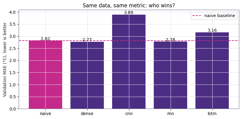
Best model: dense  (2.77 °C vs naive 2.82 °C)

Discuss: which models beat the naive baseline, and by how much? On an easy, short-horizon forecast like this one, the gap can be small, because persistence is already a strong predictor when temperature changes slowly. That is not a failure of the notebook: it is an honest and important result, and it previews two ideas that return later in the week (Thursday’s evaluation session and Friday’s ethics session): always check that a model actually beats the trivial answer before trusting it.

8 - Visualizing the predictions

A single MAE number hides where a model does well or poorly. Plotting predictions against the actual values over time shows whether the model tracks slow trends, sharp turns, or both.

model_lookup = {"dense": dense, "cnn": cnn, "rnn": rnn, "lstm": lstm}
best_model = model_lookup[best]

xb, yb = next(iter(val_ds))
pred = best_model.predict(xb, verbose=0)[:, 0]

plt.figure(figsize=(11, 4))
plt.plot((yb.numpy()[:120]*sd+mu), label="actual", color=UW_PURPLE, lw=2)
plt.plot((pred[:120]*sd+mu), label=f"{best} prediction", color=UW_GOLD, lw=2)
plt.ylabel("°C"); plt.xlabel("validation sample")
plt.title(f"{best.upper()}: predicted vs. actual temperature ({DELAY}h ahead)")
plt.legend(); plt.tight_layout(); plt.show()

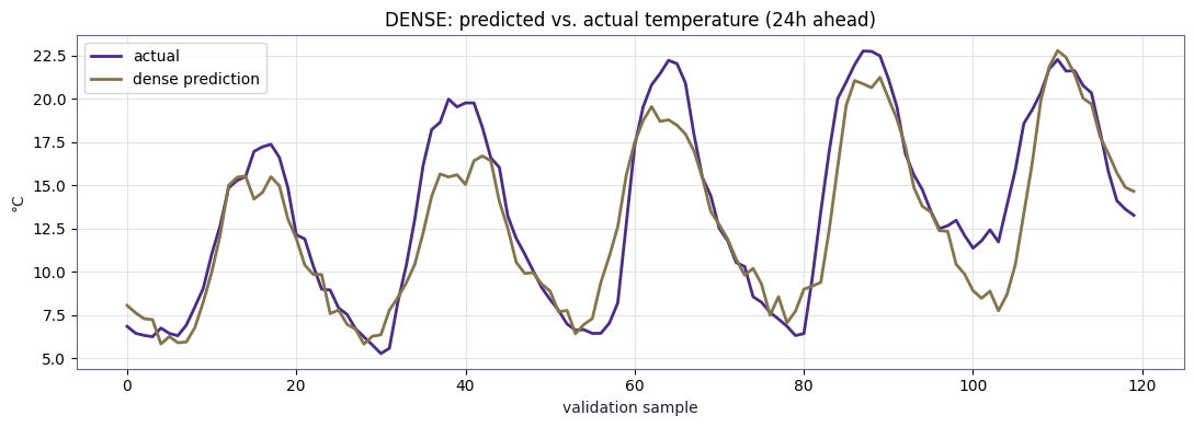
9 - Your turn

Pick one or more of the options below, then re-run section 7 to see how the comparison changes.

1. Go bidirectional. Wrap the LSTM in layers.Bidirectional(...). A bidirectional RNN runs two copies of the recurrent layer, one reading the sequence forward and one reading it backward, and combines their hidden states at each step. Every position can then use context from both before and after it (see the diagram and the caveat below).

   
   

   A bidirectional LSTM applies the same idea to LSTM cells: a forward LSTM reads the sequence left to right and a separate backward LSTM reads it right to left, and at each step their two hidden states are combined into the output. Every position then uses context from both directions.

   Diagram recreated after Figure 2 of Jian et al., “SA-Bi-LSTM: Self Attention With Bi-Directional LSTM-Based Intelligent Model for Accurate Fake News Detection,” IEEE Access, 2024 (CC BY 4.0). ieeexplore.ieee.org/document/10483072

2. Go deeper. Stack two LSTMs; the first one needs return_sequences=True so it outputs a hidden state at every timestep (not just the last one) for the second LSTM to consume.

3. Change the window. Try SEQ_LEN = 120 (5 days of history) or DELAY = 6 (predict 6 hours ahead instead of 24), and re-run from section 3 onward.

# 1) Bidirectional LSTM: wrap an LSTM in layers.Bidirectional(...)
bilstm = keras.Sequential([
    keras.Input(shape=(SEQ_LEN, N_FEAT)),
    # TODO: layers.Bidirectional( an LSTM with 32 units ),
    ...
    layers.Dense(1),
])
train_and_score(bilstm, "bilstm")

# 2) Stacked LSTM: first LSTM needs return_sequences=True
stacked = keras.Sequential([
    keras.Input(shape=(SEQ_LEN, N_FEAT)),
    # TODO: two LSTM layers (32 units). The FIRST needs return_sequences=True.
    ...
    layers.Dense(1),
])
train_and_score(stacked, "stacked")

Hint for both models

Bidirectional LSTM
layers.Bidirectional(layers.LSTM(32)),
Stacked LSTM (the first LSTM returns a sequence for the second to read)
layers.LSTM(32, return_sequences=True),
layers.LSTM(32),

Note: the bidirectional trap. A Bi-LSTM may score better here, but a real-time forecast does not have access to the future. Reading tomorrow’s data to predict tomorrow’s temperature is a form of data leakage: the model looks like it performs well, but the setup it was evaluated on could never happen in deployment. Notice it, and think about what “having the whole sequence” actually requires for your own project.

# Re-draw the comparison with your new models included:
names = list(results.keys()); vals = [results[k] for k in names]
colors = [UW_PINK if k=="naive" else UW_PURPLE for k in names]
plt.figure(figsize=(9,4))
bars = plt.bar(names, vals, color=colors)
plt.axhline(results["naive"], color=UW_PINK, ls="--", lw=1.5)
for b,v in zip(bars,vals): plt.text(b.get_x()+b.get_width()/2, v+0.02, f"{v:.2f}", ha="center", fontsize=9)
plt.ylabel("Validation MAE (°C)"); plt.title("Full ladder"); plt.tight_layout(); plt.show()

10 - Takeaways

• A sequence is defined by order and variable length, and that is exactly what today’s models are built to exploit.

• Always build a naive baseline first. It keeps every later result honest.

• 1-D CNNs detect local patterns using weight sharing across a small window. RNNs and LSTMs carry a hidden state across steps, and LSTMs specifically protect long-range memory using gates. Bidirectional models read the sequence in both directions, which requires the whole sequence in advance, so they are not appropriate for real-time forecasting.

• The same (window -> target) framing used here for forecasting also applies to anomaly detection, classifying a time window, and other tasks.

Looking ahead to tomorrow

RNNs and LSTMs read a sequence one step at a time. That is slow (it cannot be parallelized across time) and it still strains on very long sequences. Tomorrow’s session introduces the idea that addresses both limitations: attention, and the architecture built around it, the Transformer. Bidirectional processing also returns tomorrow at a much larger scale, in a model called BERT.

University of Washington, eScience Institute. See you tomorrow for transformers.